computeMatrix
This tool summarizes and prepares an intermediate file containing scores associated with genomic regions. This file can be used to plot a heatmap or profile. Typically, these genomic regions are genes, but any other regions defined in a BED format can be used. This tool can also be used to filter and sort regions according to their score.
To learn more about the specific parameters type:
computeMatrix reference-point –help or computeMatrix scale-regions –help
usage: computeMatrix [-h] [--version] ...
- optional arguments
--version show program’s version number and exit - Commands
Undocumented
Possible choices: scale-regions, reference-point
- Sub-commands:
- scale-regions
In the scale-regions mode, all regions in the BED file are stretched or shrunk to the length (in bases) indicated by the user.
usage: An example usage is:
  computeMatrix -S <biwig file> -R <bed file> -b 1000
- Required arguments
--regionsFileName, -R File name, in BED format, containing the regions to plot. If multiple bed files are given, each one is considered a group that can be plotted separately. Also, adding a “#” symbol in the bed file causes all the regions until the previous “#” to be considered one group. --scoreFileName, -S bigWig file(s) containing the scores to be plotted. BigWig files can be obtained by using the bamCoverage or bamCompare tools. More information about the bigWig file format can be found at http://genome.ucsc.edu/goldenPath/help/bigWig.html - Output options
--outFileName, -out File name to save the gzipped matrix file needed by the “plotHeatmap” and “plotProfile” tools. --outFileNameMatrix If this option is given, then the matrix of values underlying the heatmap will be saved using the indicated name, e.g. IndividualValues.tab.This matrix can easily be loaded into R or other programs. --outFileSortedRegions File name in which the regions are saved after skiping zeros or min/max threshold values. The order of the regions in the file follows the sorting order selected. This is useful, for example, to generate other heatmaps keeping the sorting of the first heatmap. Example: Heatmap1sortedRegions.bed - Optional arguments
--version show program’s version number and exit --regionBodyLength=1000, -m=1000 Distance in bases to which all regions will be fit. --startLabel=TSS Label shown in the plot for the start of the region. Default is TSS (transcription start site), but could be changed to anything, e.g. “peak start”. Note that this is only useful if you plan to plot the results yourself and not, for example, with plotHeatmap, which will override this. --endLabel=TES Label shown in the plot for the region end. Default is TES (transcription end site). See the –startLabel option for more information. --beforeRegionStartLength=0, -b=0, --upstream=0 Distance upstream of the start site of the regions defined in the region file. If the regions are genes, this would be the distance upstream of the transcription start site. --afterRegionStartLength=0, -a=0, --downstream=0 Distance downstream of the end site of the given regions. If the regions are genes, this would be the distance downstream of the transcription end site. --binSize=10, -bs=10 Length, in bases, of the non-overlapping bins for averaging the score over the regions length. --sortRegions=no Whether the output file should present the regions sorted. The default is to not sort the regions. Note that this is only useful if you plan to plot the results yourself and not, for example, with plotHeatmap, which will override this.
Possible choices: descend, ascend, no
--sortUsing=mean Indicate which method should be used for sorting. The value is computed for each row.
Possible choices: mean, median, max, min, sum, region_length
--averageTypeBins=mean Define the type of statistic that should be used over the bin size range. The options are: “mean”, “median”, “min”, “max”, “sum” and “std”. The default is “mean”.
Possible choices: mean, median, min, max, std, sum
--missingDataAsZero=False If set, missing data (NAs) will be treated as zeros. The default is to ignore such cases, which will be depicted as black areas in a heatmap. (see the –missingDataColor argument of the plotHeatmap command for additional options). --skipZeros=False Whether regions with only scores of zero should be included or not. Default is to include them. --minThreshold Numeric value. Any region containing a value that is less than or equal to this will be skipped. This is useful to skip, for example, genes where the read count is zero for any of the bins. This could be the result of unmappable areas and can bias the overall results. --maxThreshold Numeric value. Any region containing a value greater than or equal to this will be skipped. The maxThreshold is useful to skip those few regions with very high read counts (e.g. micro satellites) that may bias the average values. --quiet=False, -q=False Set to remove any warning or processing messages. --scale=1 If set, all values are multiplied by this number. --numberOfProcessors=max/2, -p=max/2 Number of processors to use. Type “max/2” to use half the maximum number of processors or “max” to use all available processors.
- reference-point
Reference-point refers to a position within a BED region (e.g., the starting point). In this mode, only those genomicpositions before (upstream) and/or after (downstream) of the reference point will be plotted.
usage: An example usage is:
  computeMatrix -S <biwig file> -R <bed file> -a 3000 -b 3000
- Required arguments
--regionsFileName, -R File name, in BED format, containing the regions to plot. If multiple bed files are given, each one is considered a group that can be plotted separately. Also, adding a “#” symbol in the bed file causes all the regions until the previous “#” to be considered one group. --scoreFileName, -S bigWig file(s) containing the scores to be plotted. BigWig files can be obtained by using the bamCoverage or bamCompare tools. More information about the bigWig file format can be found at http://genome.ucsc.edu/goldenPath/help/bigWig.html - Output options
--outFileName, -out File name to save the gzipped matrix file needed by the “plotHeatmap” and “plotProfile” tools. --outFileNameMatrix If this option is given, then the matrix of values underlying the heatmap will be saved using the indicated name, e.g. IndividualValues.tab.This matrix can easily be loaded into R or other programs. --outFileSortedRegions File name in which the regions are saved after skiping zeros or min/max threshold values. The order of the regions in the file follows the sorting order selected. This is useful, for example, to generate other heatmaps keeping the sorting of the first heatmap. Example: Heatmap1sortedRegions.bed - Optional arguments
--version show program’s version number and exit --referencePoint=TSS The reference point for the plotting could be either the region start (TSS), the region end (TES) or the center of the region. Note that regardless of what you specify, plotHeatmap/plotProfile will default to using “TSS” as the label.
Possible choices: TSS, TES, center
--beforeRegionStartLength=500, -b=500, --upstream=500 Distance upstream of the reference-point selected. --afterRegionStartLength=1500, -a=1500, --downstream=1500 Distance downstream of the reference-point selected. --nanAfterEnd=False If set, any values after the region end are discarded. This is useful to visualize the region end when not using the scale-regions mode and when the reference-point is set to the TSS. --binSize=10, -bs=10 Length, in bases, of the non-overlapping bins for averaging the score over the regions length. --sortRegions=no Whether the output file should present the regions sorted. The default is to not sort the regions. Note that this is only useful if you plan to plot the results yourself and not, for example, with plotHeatmap, which will override this.
Possible choices: descend, ascend, no
--sortUsing=mean Indicate which method should be used for sorting. The value is computed for each row.
Possible choices: mean, median, max, min, sum, region_length
--averageTypeBins=mean Define the type of statistic that should be used over the bin size range. The options are: “mean”, “median”, “min”, “max”, “sum” and “std”. The default is “mean”.
Possible choices: mean, median, min, max, std, sum
--missingDataAsZero=False If set, missing data (NAs) will be treated as zeros. The default is to ignore such cases, which will be depicted as black areas in a heatmap. (see the –missingDataColor argument of the plotHeatmap command for additional options). --skipZeros=False Whether regions with only scores of zero should be included or not. Default is to include them. --minThreshold Numeric value. Any region containing a value that is less than or equal to this will be skipped. This is useful to skip, for example, genes where the read count is zero for any of the bins. This could be the result of unmappable areas and can bias the overall results. --maxThreshold Numeric value. Any region containing a value greater than or equal to this will be skipped. The maxThreshold is useful to skip those few regions with very high read counts (e.g. micro satellites) that may bias the average values. --quiet=False, -q=False Set to remove any warning or processing messages. --scale=1 If set, all values are multiplied by this number. --numberOfProcessors=max/2, -p=max/2 Number of processors to use. Type “max/2” to use half the maximum number of processors or “max” to use all available processors.
- An example usage is:
- computeMatrix reference-point -S <bigwig file> -R <bed file> -b 1000
Usage Example:
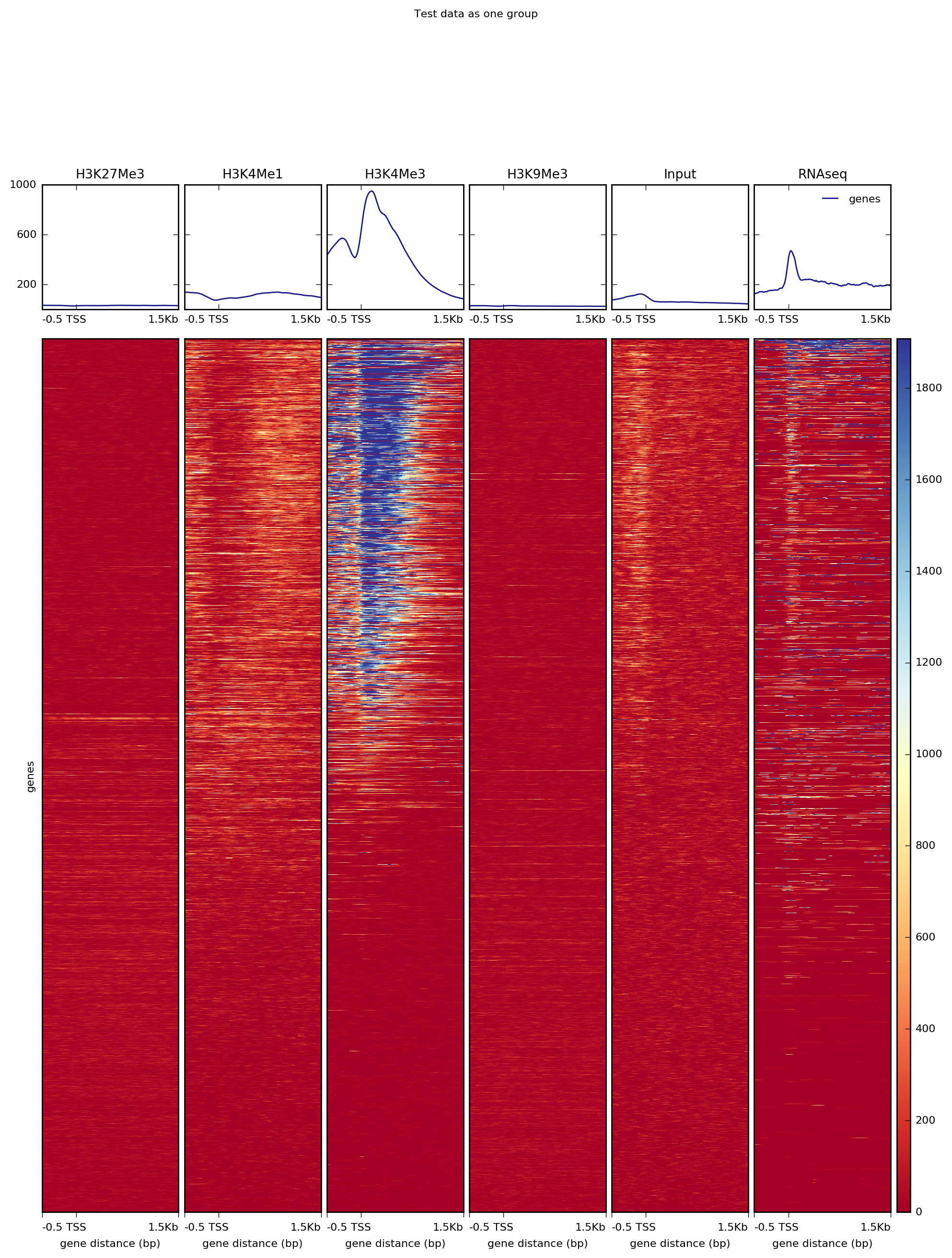
computeMatrix has two main modes of use: for computing the signal distribution relative to a point (“reference-point”) and for computing the signal over a region (“scale-regions”). The “reference-point” method is commonly used before plotting the signal around the transcription start site. An example of that with our test ENCODE dataset is depicted below:
computeMatrix reference-point \
    -q --skipZeros \
    -S *.bigWig \
    -R genes.bed \
    -out matrix_one_group_TSS.gz

plotHeatmap -m matrix_one_group_TSS.gz \
    -out ExampleComputeMatrix1.png \
    --plotTitle "Test data as one group"
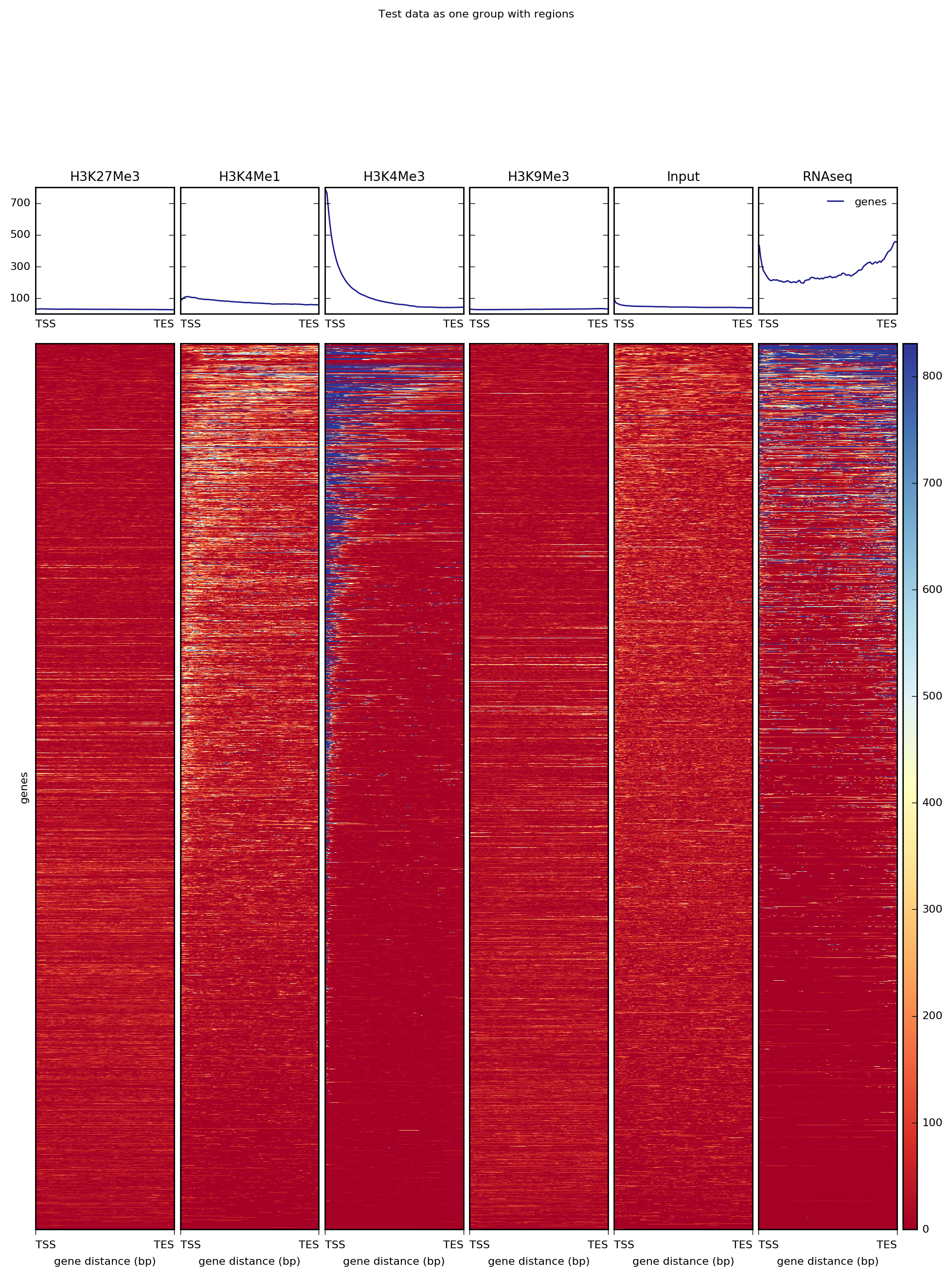
Alternatively, for RNAseq and many other ChIP signals it’s more informative to plot the signal distribution over exons or other feature types. For such cases, one can use the “scale-regions” method.
computeMatrix scale-regions \
    -q --skipZeros \
    -S *.bigWig \
    -R genes.bed \
    -out matrix_one_group.gz

plotHeatmap -m matrix_one_group.gz \
    -out ExampleComputeMatrix2.png \
    --plotTitle "Test data as one group with regions"
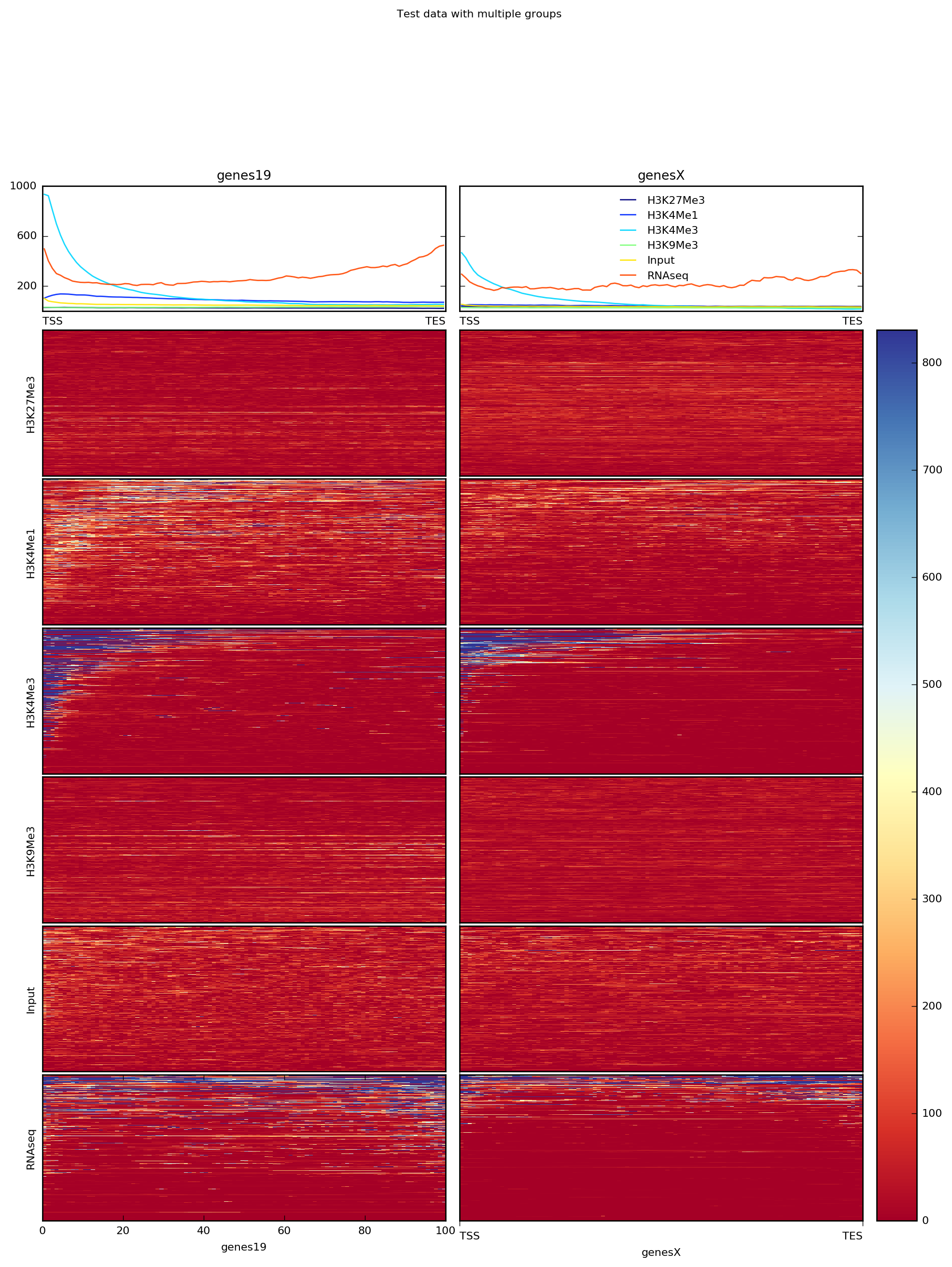
It’s often the case that one has multiple groups of regions to consider per sample. For such cases, you can simply specify multiple BED files (in this case, we’ve split the BED file by chromosome).
computeMatrix scale-regions \
    -q --skipZeros \
    -S *.bigWig \
    -R genes19.bed genesX.bed \
    -out matrix_two_groups.gz

plotHeatmap -m matrix_two_groups.gz \
    -out ExampleComputeMatrix3.png \
    --perGroup \
    --plotTitle "Test data with multiple groups"
Note that computeMatrix can use multiple threads, which significantly decreases the time required.