computeMatrix
This tool calculates scores per genome regions and prepares an intermediate file that can be used with plotHeatmap and plotProfiles.
Typically, the genome regions are genes, but any other regions defined in a BED file can be used.
computeMatrix accepts multiple score files (bigWig format) and multiple regions files (BED format).
This tool can also be used to filter and sort regions according
to their score.
To learn more about the specific parameters, type:
$ computeMatrix reference-point –help or
$ computeMatrix scale-regions –help
usage: computeMatrix [-h] [--version] ...
Named Arguments
- --version
show program’s version number and exit
Commands
Possible choices: scale-regions, reference-point
Sub-commands
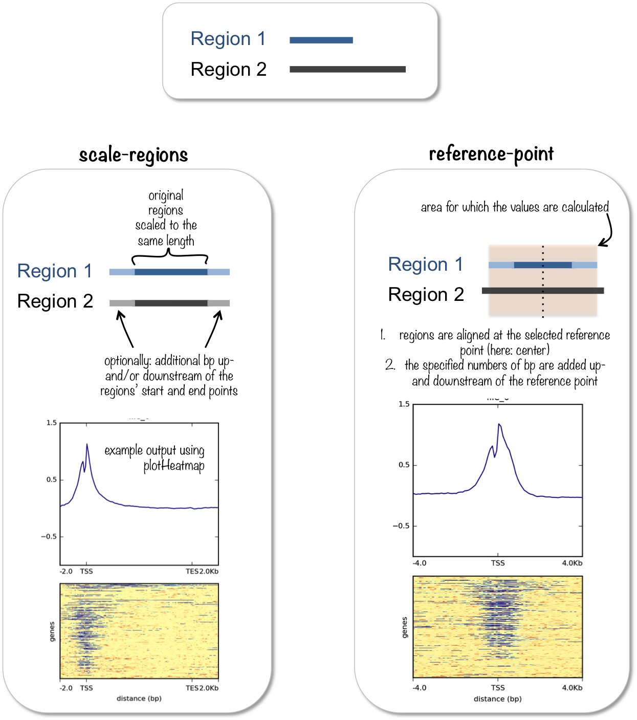
scale-regions
In the scale-regions mode, all regions in the BED file are stretched or shrunken to the length (in bases) indicated by the user.
An example usage is:
  computeMatrix scale-regions -S <biwig file(s)> -R <bed file> -b 1000
Required arguments
- --regionsFileName, -R
File name or names, in BED or GTF format, containing the regions to plot. If multiple bed files are given, each one is considered a group that can be plotted separately. Also, adding a “#” symbol in the bed file causes all the regions until the previous “#” to be considered one group.
- --scoreFileName, -S
bigWig file(s) containing the scores to be plotted. Multiple files should be separated by spaced. BigWig files can be obtained by using the bamCoverage or bamCompare tools. More information about the bigWig file format can be found at http://genome.ucsc.edu/goldenPath/help/bigWig.html
Output options
- --outFileName, -out, -o
File name to save the gzipped matrix file needed by the “plotHeatmap” and “plotProfile” tools.
- --outFileNameMatrix
If this option is given, then the matrix of values underlying the heatmap will be saved using the indicated name, e.g. IndividualValues.tab.This matrix can easily be loaded into R or other programs.
- --outFileSortedRegions
File name in which the regions are saved after skiping zeros or min/max threshold values. The order of the regions in the file follows the sorting order selected. This is useful, for example, to generate other heatmaps keeping the sorting of the first heatmap. Example: Heatmap1sortedRegions.bed
Optional arguments
- --version
show program’s version number and exit
- --regionBodyLength, -m
Distance in bases to which all regions will be fit. (Default: 1000)
- --startLabel
Label shown in the plot for the start of the region. Default is TSS (transcription start site), but could be changed to anything, e.g. “peak start”. Note that this is only useful if you plan to plot the results yourself and not, for example, with plotHeatmap, which will override this. (Default: “TSS”)
- --endLabel
Label shown in the plot for the region end. Default is TES (transcription end site). See the –startLabel option for more information. (Default: “TES”)
- --beforeRegionStartLength, -b, --upstream
Distance upstream of the start site of the regions defined in the region file. If the regions are genes, this would be the distance upstream of the transcription start site. (Default: 0)
- --afterRegionStartLength, -a, --downstream
Distance downstream of the end site of the given regions. If the regions are genes, this would be the distance downstream of the transcription end site. (Default: 0)
- --unscaled5prime
Number of bases at the 5-prime end of the region to exclude from scaling. By default, each region is scaled to a given length (see the –regionBodyLength option). In some cases it is useful to look at unscaled signals around region boundaries, so this setting specifies the number of unscaled bases on the 5-prime end of each boundary. (Default: 0)
- --unscaled3prime
Like –unscaled5prime, but for the 3-prime end. (Default: 0)
- --binSize, -bs
Length, in bases, of the non-overlapping bins for averaging the score over the regions length. (Default: 10)
- --sortRegions
Possible choices: descend, ascend, no, keep
Whether the output file should present the regions sorted. The default is to not sort the regions. Note that this is only useful if you plan to plot the results yourself and not, for example, with plotHeatmap, which will override this. Note also that unsorted output will be in whatever order the regions happen to be processed in and not match the order in the input files. If you require the output order to match that of the input regions, then either specify “keep” or use computeMatrixOperations to resort the results file. (Default: “keep”)
- --sortUsing
Possible choices: mean, median, max, min, sum, region_length
Indicate which method should be used for sorting. The value is computed for each row.Note that the region_length option will lead to a dotted line within the heatmap that indicates the end of the regions. (Default: “mean”)
- --sortUsingSamples
List of sample numbers (order as in matrix), that are used for sorting by –sortUsing, no value uses all samples, example: –sortUsingSamples 1 3
- --averageTypeBins
Possible choices: mean, median, min, max, std, sum
Define the type of statistic that should be used over the bin size range. The options are: “mean”, “median”, “min”, “max”, “sum” and “std”. The default is “mean”. (Default: “mean”)
- --missingDataAsZero
If set, missing data (NAs) will be treated as zeros. The default is to ignore such cases, which will be depicted as black areas in a heatmap. (see the –missingDataColor argument of the plotHeatmap command for additional options).
- --skipZeros
Whether regions with only scores of zero should be included or not. Default is to include them.
- --minThreshold
Numeric value. Any region containing a value that is less than or equal to this will be skipped. This is useful to skip, for example, genes where the read count is zero for any of the bins. This could be the result of unmappable areas and can bias the overall results. (Default: None)
- --maxThreshold
Numeric value. Any region containing a value greater than or equal to this will be skipped. The maxThreshold is useful to skip those few regions with very high read counts (e.g. micro satellites) that may bias the average values. (Default: None)
- --blackListFileName, -bl
A BED file containing regions that should be excluded from all analyses. Currently this works by rejecting genomic chunks that happen to overlap an entry. Consequently, for BAM files, if a read partially overlaps a blacklisted region or a fragment spans over it, then the read/fragment might still be considered.
- --samplesLabel
Labels for the samples. This will then be passed to plotHeatmap and plotProfile. The default is to use the file name of the sample. The sample labels should be separated by spaces and quoted if a label itselfcontains a space E.g. –samplesLabel label-1 “label 2”
- --smartLabels
Instead of manually specifying labels for the input bigWig and BED/GTF files, this causes deepTools to use the file name after removing the path and extension.
- --quiet, -q
Set to remove any warning or processing messages.
- --verbose
Being VERY verbose in the status messages. –quiet will disable this.
- --scale
If set, all values are multiplied by this number. (Default: 1)
- --numberOfProcessors, -p
Number of processors to use. Type “max/2” to use half the maximum number of processors or “max” to use all available processors. (Default: 1)
GTF/BED12 options
- --metagene
When either a BED12 or GTF file are used to provide regions, perform the computation on the merged exons, rather than using the genomic interval defined by the 5-prime and 3-prime most transcript bound (i.e., columns 2 and 3 of a BED file). If a BED3 or BED6 file is used as input, then columns 2 and 3 are used as an exon. (Default: False)
- --transcriptID
When a GTF file is used to provide regions, only entries with this value as their feature (column 3) will be processed as transcripts. (Default: “transcript”)
- --exonID
When a GTF file is used to provide regions, only entries with this value as their feature (column 3) will be processed as exons. CDS would be another common value for this. (Default: “exon”)
- --transcript_id_designator
Each region has an ID (e.g., ACTB) assigned to it, which for BED files is either column 4 (if it exists) or the interval bounds. For GTF files this is instead stored in the last column as a key:value pair (e.g., as ‘transcript_id “ACTB”’, for a key of transcript_id and a value of ACTB). In some cases it can be convenient to use a different identifier. To do so, set this to the desired key. (Default: “transcript_id”)
reference-point
Reference-point refers to a position within a BED region (e.g., the starting point). In this mode, only those genomicpositions before (upstream) and/or after (downstream) of the reference point will be plotted.
An example usage is:
  computeMatrix reference-point -S <biwig file(s)> -R <bed file> -a 3000 -b 3000
Required arguments
- --regionsFileName, -R
File name or names, in BED or GTF format, containing the regions to plot. If multiple bed files are given, each one is considered a group that can be plotted separately. Also, adding a “#” symbol in the bed file causes all the regions until the previous “#” to be considered one group.
- --scoreFileName, -S
bigWig file(s) containing the scores to be plotted. Multiple files should be separated by spaced. BigWig files can be obtained by using the bamCoverage or bamCompare tools. More information about the bigWig file format can be found at http://genome.ucsc.edu/goldenPath/help/bigWig.html
Output options
- --outFileName, -out, -o
File name to save the gzipped matrix file needed by the “plotHeatmap” and “plotProfile” tools.
- --outFileNameMatrix
If this option is given, then the matrix of values underlying the heatmap will be saved using the indicated name, e.g. IndividualValues.tab.This matrix can easily be loaded into R or other programs.
- --outFileSortedRegions
File name in which the regions are saved after skiping zeros or min/max threshold values. The order of the regions in the file follows the sorting order selected. This is useful, for example, to generate other heatmaps keeping the sorting of the first heatmap. Example: Heatmap1sortedRegions.bed
Optional arguments
- --version
show program’s version number and exit
- --referencePoint
Possible choices: TSS, TES, center
The reference point for the plotting could be either the region start (TSS), the region end (TES) or the center of the region. Note that regardless of what you specify, plotHeatmap/plotProfile will default to using “TSS” as the label. (Default: “TSS”)
- --beforeRegionStartLength, -b, --upstream
Distance upstream of the reference-point selected. (Default: 500)
- --afterRegionStartLength, -a, --downstream
Distance downstream of the reference-point selected. (Default: 1500)
- --nanAfterEnd
If set, any values after the region end are discarded. This is useful to visualize the region end when not using the scale-regions mode and when the reference-point is set to the TSS.
- --binSize, -bs
Length, in bases, of the non-overlapping bins for averaging the score over the regions length. (Default: 10)
- --sortRegions
Possible choices: descend, ascend, no, keep
Whether the output file should present the regions sorted. The default is to not sort the regions. Note that this is only useful if you plan to plot the results yourself and not, for example, with plotHeatmap, which will override this. Note also that unsorted output will be in whatever order the regions happen to be processed in and not match the order in the input files. If you require the output order to match that of the input regions, then either specify “keep” or use computeMatrixOperations to resort the results file. (Default: “keep”)
- --sortUsing
Possible choices: mean, median, max, min, sum, region_length
Indicate which method should be used for sorting. The value is computed for each row.Note that the region_length option will lead to a dotted line within the heatmap that indicates the end of the regions. (Default: “mean”)
- --sortUsingSamples
List of sample numbers (order as in matrix), that are used for sorting by –sortUsing, no value uses all samples, example: –sortUsingSamples 1 3
- --averageTypeBins
Possible choices: mean, median, min, max, std, sum
Define the type of statistic that should be used over the bin size range. The options are: “mean”, “median”, “min”, “max”, “sum” and “std”. The default is “mean”. (Default: “mean”)
- --missingDataAsZero
If set, missing data (NAs) will be treated as zeros. The default is to ignore such cases, which will be depicted as black areas in a heatmap. (see the –missingDataColor argument of the plotHeatmap command for additional options).
- --skipZeros
Whether regions with only scores of zero should be included or not. Default is to include them.
- --minThreshold
Numeric value. Any region containing a value that is less than or equal to this will be skipped. This is useful to skip, for example, genes where the read count is zero for any of the bins. This could be the result of unmappable areas and can bias the overall results. (Default: None)
- --maxThreshold
Numeric value. Any region containing a value greater than or equal to this will be skipped. The maxThreshold is useful to skip those few regions with very high read counts (e.g. micro satellites) that may bias the average values. (Default: None)
- --blackListFileName, -bl
A BED file containing regions that should be excluded from all analyses. Currently this works by rejecting genomic chunks that happen to overlap an entry. Consequently, for BAM files, if a read partially overlaps a blacklisted region or a fragment spans over it, then the read/fragment might still be considered.
- --samplesLabel
Labels for the samples. This will then be passed to plotHeatmap and plotProfile. The default is to use the file name of the sample. The sample labels should be separated by spaces and quoted if a label itselfcontains a space E.g. –samplesLabel label-1 “label 2”
- --smartLabels
Instead of manually specifying labels for the input bigWig and BED/GTF files, this causes deepTools to use the file name after removing the path and extension.
- --quiet, -q
Set to remove any warning or processing messages.
- --verbose
Being VERY verbose in the status messages. –quiet will disable this.
- --scale
If set, all values are multiplied by this number. (Default: 1)
- --numberOfProcessors, -p
Number of processors to use. Type “max/2” to use half the maximum number of processors or “max” to use all available processors. (Default: 1)
GTF/BED12 options
- --metagene
When either a BED12 or GTF file are used to provide regions, perform the computation on the merged exons, rather than using the genomic interval defined by the 5-prime and 3-prime most transcript bound (i.e., columns 2 and 3 of a BED file). If a BED3 or BED6 file is used as input, then columns 2 and 3 are used as an exon. (Default: False)
- --transcriptID
When a GTF file is used to provide regions, only entries with this value as their feature (column 3) will be processed as transcripts. (Default: “transcript”)
- --exonID
When a GTF file is used to provide regions, only entries with this value as their feature (column 3) will be processed as exons. CDS would be another common value for this. (Default: “exon”)
- --transcript_id_designator
Each region has an ID (e.g., ACTB) assigned to it, which for BED files is either column 4 (if it exists) or the interval bounds. For GTF files this is instead stored in the last column as a key:value pair (e.g., as ‘transcript_id “ACTB”’, for a key of transcript_id and a value of ACTB). In some cases it can be convenient to use a different identifier. To do so, set this to the desired key. (Default: “transcript_id”)
- An example usage is:
computeMatrix reference-point -S <bigwig file(s)> -R <bed file(s)> -b 1000
Details
computeMatrix has two main modes of use:
for computing the signal distribution relative to a point (
reference-point), e.g., the beginning or end of each genomic regionfor computing the signal over a set of regions (
scale-regions) where all regions are scaled to the same size
computeMatrix is tightly connected to plotHeatmap and plotProfile: it takes the values of all the signal files and all genomic regions that you would like to plot and computes the corresponding data matrix.
See plotHeatmap and plotProfile for example plots.
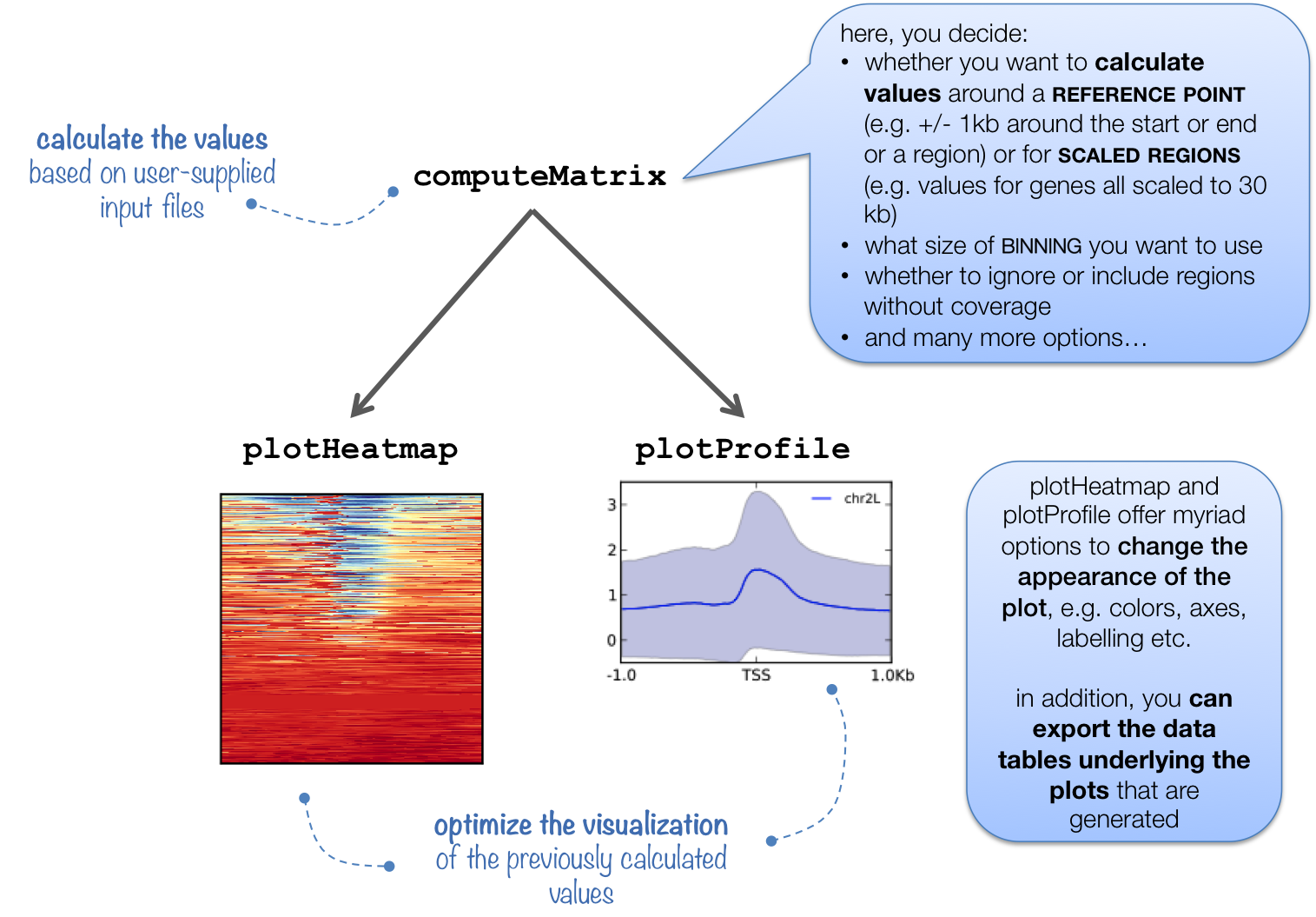
In addition to generating the intermediate, gzipped file for plotHeatmap and plotProfile, computeMatrix can also be used to simply output the values underlying the heatmap or to filter and sort BED files using, for example, the --skipZeros and the --sortUsing parameters.
The following tables summarizes the kinds of optional outputs that are available with the three tools.
optional output type |
command |
computeMatrix |
plotHeatmap |
plotProfile |
values underlying the heatmap |
|
yes |
yes |
no |
values underlying the profile |
|
no |
yes |
yes |
sorted and/or filtered regions |
|
yes |
yes |
yes |
Tip
computeMatrix can use multiple threads (-p option), which significantly decreases the time for calculating the values.
Attention
As of version 3.0, computeMatrix produces output with labels present for each sample. Matrices produced with that or later versions can not be used with older versions of plotHeatmap or any other deepTools program.
Note
computeMatrix will properly handle strand information if your BED file includes that column (GTF files always include strand). For the --metagene option to work, you will need either a BED12 (including columns 11 and 12) or a GTF file as input. GFF is NOT the same as GTF format!
Examples
The following examples should give you an idea of some of the most often used settings for computeMatrix. As you can see, computeMatrix offers myriad tweaks and may turn out to be more useful to you than “just” to calculate heatmap matrices.
Example 1: single input files (reference-point mode)
Here, we start with a single bigWig and a single BED file, i.e., computeMatrix will:
take the beginning of the regions specified in the BED file
add the values indicated with
--beforeRegionStartLength(-b) and--afterRegionStartLength(-a)split the resulting region up into 50 bp bins (can be changed via (
--binSize)calculate the mean score based on the scores given in the bigWig file (the kind of score can be changed via
--averageTypeBins)write out the values where each row corresponds to one region in the BED file (note that you can, for example, skip regions with zero coverage; sorting is also possible)
$ computeMatrix reference-point \ # choose the mode
       --referencePoint TSS \ # alternatives: TES, center
       -b 3000 -a 10000 \ # define the region you are interested in
       -R testFiles/genes.bed \
       -S testFiles/log2ratio_H3K4Me3_chr19.bw  \
       --skipZeros \
       -o matrix1_H3K4me3_l2r_TSS.gz \ # to be used with plotHeatmap and plotProfile
       --outFileSortedRegions regions1_H3K4me3_l2r_genes.bed
Let’s have a closer look at the regions’ output:
$ wc -l testFiles/genes.bed # original file
   18257 testFiles/genes.bed
$ wc -l regions1_H3K4me3_l2r_genes.bed # file generated by computeMatrix
   12423 regions1_H3K4me3_l2r_genes.bed
As you can see, the number of regions is drastically reduced. The remaining genes happen to be the ones on chromosome 19 for which there was at least one overlapping read. This makes sense since the bigWig file used above only contained reads for chromosome 19.
# the original file contained genes for chr.19 and chr.X
$ cut -f 1 testFiles/genes.bed | sort | uniq -c
    12439 19
    5818 X

# the regions used for the computation of the matrix for the heatmap are all located on chr.19 due to the --skipZeros setting (see above)
$ cut -f 1 regions1_H3K4me3_l2r_genes.bed | sort | uniq -c
    1 #genes
    12422 19
Example 2: multiple input files (scale-regions mode)
$ deepTools2.0/bin/computeMatrix scale-regions \
  -R genes_chr19_firstHalf.bed genes_chr19_secondHalf.bed \ # separate multiple files with spaces
  -S testFiles/log2ratio_*.bw  \ or use the wild card approach
  -b 3000 -a 3000 \
  --regionBodyLength 5000 \
  --skipZeros -o matrix2_multipleBW_l2r_twoGroups_scaled.gz \
  --outFileNameMatrix matrix2_multipleBW_l2r_twoGroups_scaled.tab \
  --outFileSortedRegions regions2_multipleBW_l2r_twoGroups_genes.bed
Note that the reported regions will have the same coordinates as the ones in the originally supplied file, not the region that was used for the heatmap matrix.
The groups of regions supplied by two individual files will be merged into one:
$ head -n 2 regions2_multipleBW_l2r_twoGroups_genes.bed
19  60104   70951   ENST00000592209 0.0     -       genes_chr19_firstHalf
19  60950   70966   ENST00000606728 0.0     -       genes_chr19_firstHalf

$ tail -n 3 regions2_multipleBW_l2r_twoGroups_genes.bed
19  59108549        59110722        ENST00000596427 0.0     -       genes_chr19_secondHalf
19  59110333        59110802        ENST00000464061 0.0     +       genes_chr19_secondHalf
#genes_chr19_secondHalf
Tip
More examples can be found in our Gallery.