Step-by-step protocols
- How can I do...?
- I have downloaded/received a BAM file - how do I generate a file I can look at in a genome browser?
- How can I assess the reproducibility of my sequencing replicates?
- How do I know whether my sample is GC biased? And if it is, how do I correct for it?
- How do I get an input-normalized ChIP-seq coverage file?
- How can I compare the ChIP strength for different ChIP experiments?
- How do I get a (clustered) heatmap of sequencing-depth-normalized read coverages around the transcription start site of all genes?
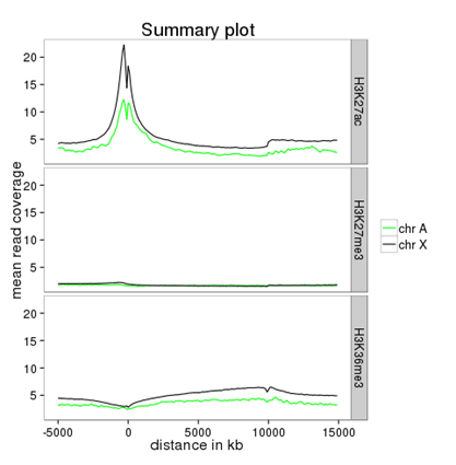
- How can I compare the average signal for X- and autosomal genes for 2 or more different sequencing experiments?
- How to obtain a BED file for X chromosomal and autosomal genes each
- Compute the average values for X and autosomal genes
How can I do...?
This section should give you a quick overview of how to do many common tasks. We’re using screenshots from Galaxy here, so if you’re using the command-line version then you can easily follow the given examples by typing the program name and the help option (e.g. /deepTools/bin/bamCoverage –help), which will show you all the parameters and options (most of them named very similarly to those in Galaxy).
For each “recipe” here, you will find the screenshot of the tool and the input parameters on the left hand side (we marked non-default, user-specified entries) and screenshots of the output on the right hand side. Do let us know if you spot things that are missing, should be explained better, or are simply confusing!
There are many more ways in which you can use deepTools Galaxy than those described here, so be creative once you’re comfortable with using them. For detailed explanations of what the tools do, follow the links.
All recipes assume that you have uploaded your files into a Galaxy instance with a deepTools installation, e.g., deepTools Galaxy
If you would like to try out the protocols with sample data, go to deepTools Galaxy –> “Shared Data” –> “Data Libraries” –> “deepTools Test Files”. Simply select BED/BAM/bigWig files and click, “to History”. You can also download the test datasets by clicking “Download” at the top.
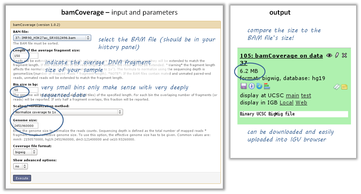
I have downloaded/received a BAM file - how do I generate a file I can look at in a genome browser?
- tool: bamCoverage
- input: your BAM file
Note: BAM files can also be viewed in genome browsers, however, they’re large and tend to freeze the applications. Generating bigWig files of read coverages will help you a lot in this regard. In addition, if you have more than one sample you’d like to look at, it is helpful to normalize all of them to 1x sequencing depth.
How can I assess the reproducibility of my sequencing replicates?
tool: multiBamSummary
- input: BAM files
- you can compare as many samples as you want, though the more you use the longer the computation will take
output: heatmap of correlations - the closer two samples are to each other, the more similar their read coverages will be

How do I know whether my sample is GC biased? And if it is, how do I correct for it?
- you need a BAM file of your sample
- use the tool computeGCBias on that BAM file (default settings, just make sure your reference genome and genome size are matching)
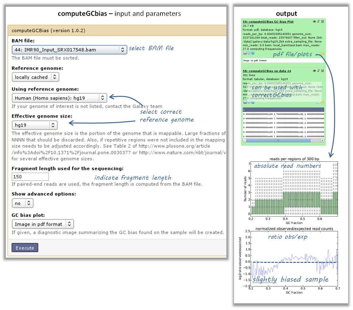
have a look at the image that is produced and compare it to the examples here
if your sample shows an almost linear increase in exp/obs coverage (on the log scale of the lower plot), then you should consider correcting the GC bias - if you think that the biological interpretation of this data would otherwise be compromised (e.g. by comparing it to another sample that does not have an inherent GC bias)
- the GC bias can be corrected with the tool correctGCBias using the second output of the computeGCbias tool that you had to run anyway
- CAUTION!! correctGCbias will add reads to otherwise depleted regions (typically GC-poor regions), that means that you should not remove duplicates in any downstream analyses based on the GC-corrected BAM file (we therefore recommend removing duplicates before doing the correction so that only those duplicate reads are kept that were produced by the GC correction procedure)

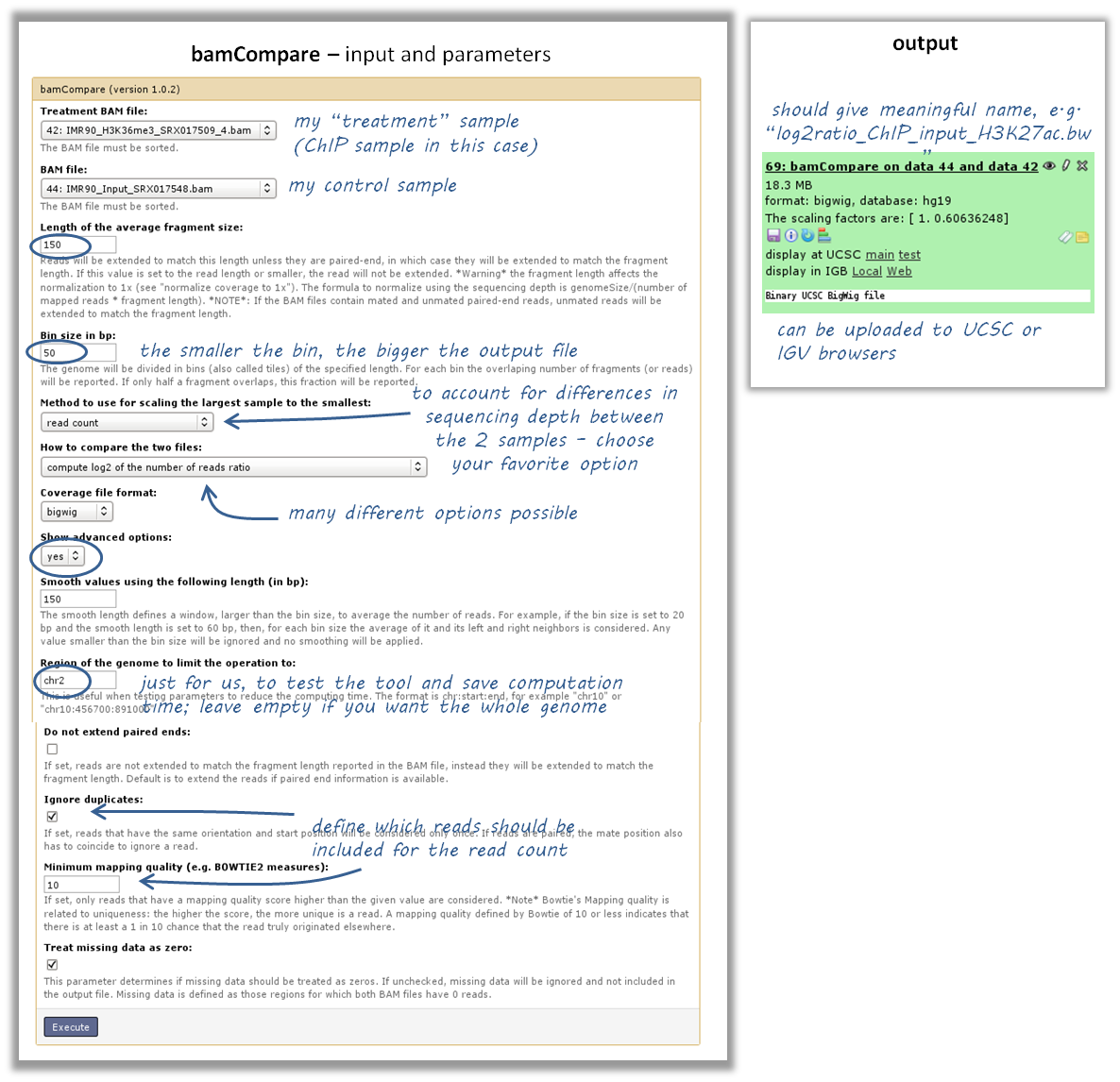
How do I get an input-normalized ChIP-seq coverage file?
- input: you need two BAM files, one for the input and one for the ChIP-seq experiment
- tool: bamCompare with ChIP = treatment, input = control sample
How can I compare the ChIP strength for different ChIP experiments?
- tool: plotFingerprint
- input: as many BAM files as you’d like to compare. Make sure you get all the labels right!

How do I get a (clustered) heatmap of sequencing-depth-normalized read coverages around the transcription start site of all genes?
tools: computeMatrix, then plotHeatmap
- inputs:
- 1 bigWig file of normalized read coverages (e.g. the result of bamCoverage or bamCompare)
- 1 BED or INTERVAL file of genes, e.g. obtained through Galaxy via “Get Data” –> “UCSC main table browser” –> group: “Genes and Gene Predictions” –> (e.g.) “RefSeqGenes” –> send to Galaxy (see screenshots below)
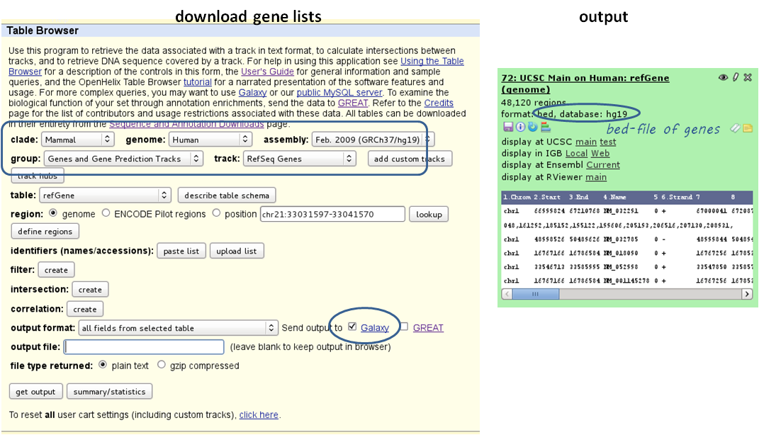
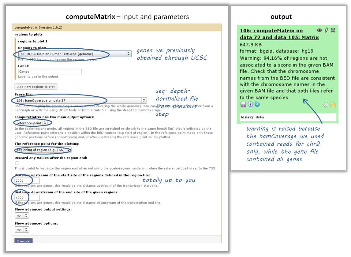
- use computeMatrix with the bigWig file and the BED file
- indicate “reference-point” (and whatever other option you would like to tune, see screenshot below)
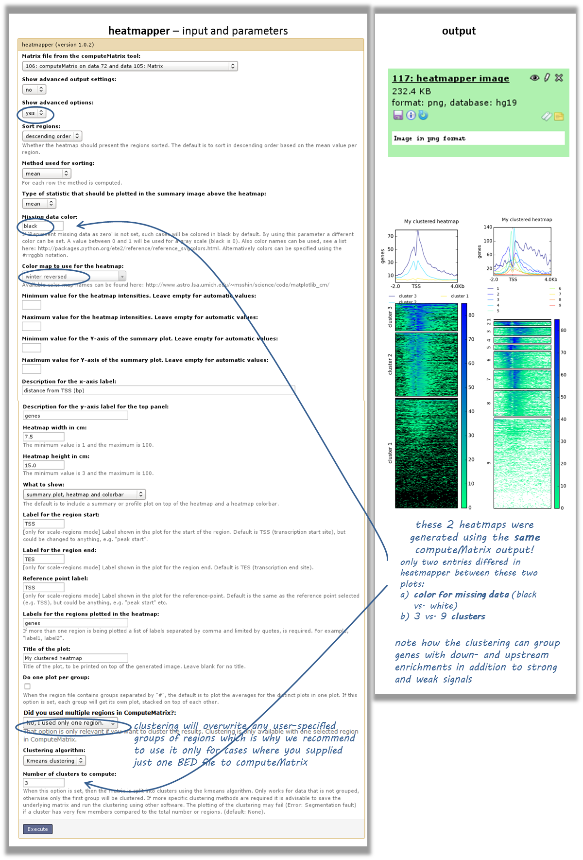
- use the output from computeMatrix with plotHeatmap
- if you would like to cluster the signals, choose “k-means clustering” (last option of “advanced options”) with a reasonable number of clusters (usually between 2 to 7)
How can I compare the average signal for X- and autosomal genes for 2 or more different sequencing experiments?
Make sure you’re familiar with computeMatrix and profiler before using this protocol.
- tools:
- Filter data on any column using simple expressions
- computeMatrix
- profiler
- (plotting the summary plots for multiple samples)
- inputs:
- several bigWig files (one for each sequencing experiment you would like to compare)
- two BED files, one with X-chromosomal and one with autosomal genes
How to obtain a BED file for X chromosomal and autosomal genes each
download a full list of genes via “Get Data” –> “UCSC main table browser” –> group:”Genes and Gene Predictions” –> tracks: (e.g.) “RefSeqGenes” –> send to Galaxy
filter the list twice using the tool “Filter data on any column using simple expressions”
- first use the expression: c1==”chrX” to filter the list of all genes –> this will generate a list of X-linked genes
- then re-run the filtering, now with c1!=”chrX”, which will generate a list of genes that do not belong to chromosome X (!= indicates “not matching”)
Compute the average values for X and autosomal genes
use computeMatrix for all of the signal files (bigWig format) at once
- supply both filtered BED files (click on “Add new regions to plot” once) and label them
- indicate the corresponding signal files
now use plotProfile on the resulting file
- important: display the “advanced output options” and select “save the data underlying the average profile” –> this will generate a table in addition to the summary plot images
